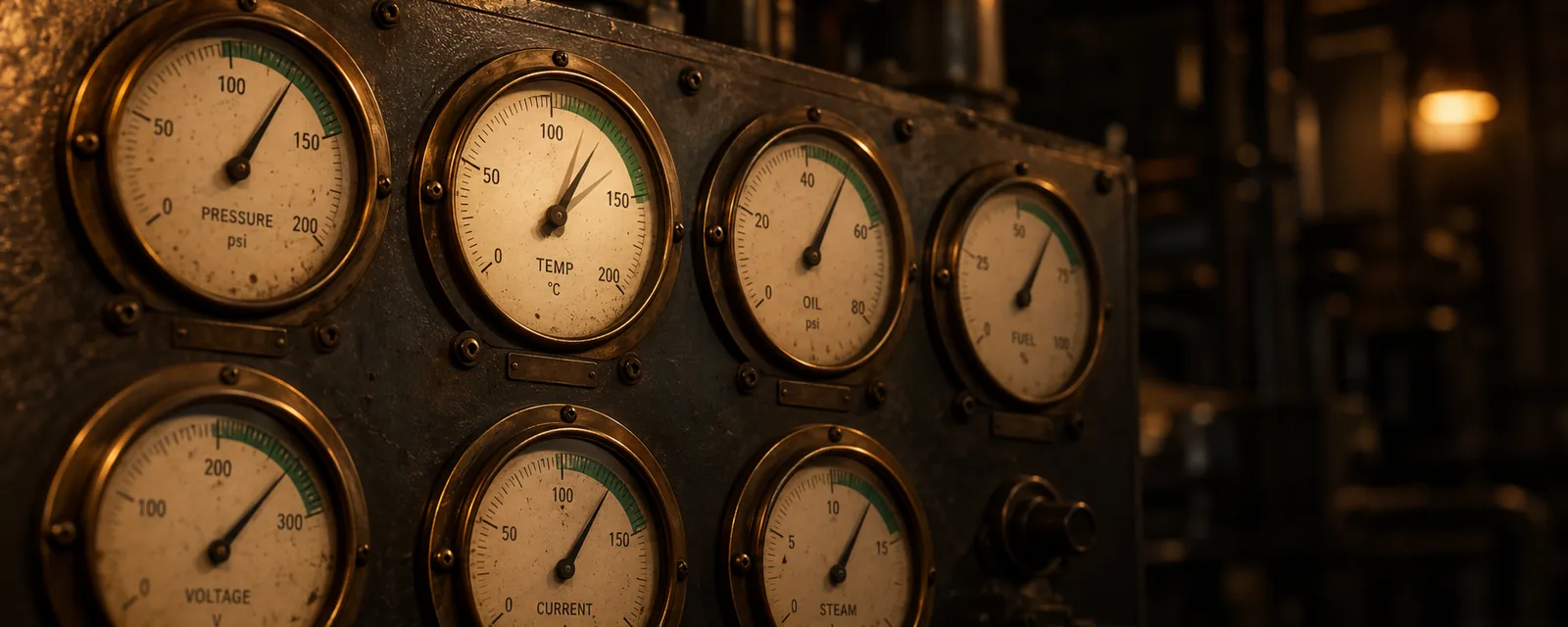
A pump can hold a steady flow and an unremarkable temperature while its controller quietly works harder to compensate for a developing restriction. To someone watching only those readings, the machine may appear unchanged. The difference lies in the relationship between output, effort and operating conditions, and it may become visible only when several observations are considered together over time. This is the kind of distinction a useful sensing system should help us recognise before the visible output begins to fail.

The question is how to learn those relationships from incomplete evidence. One approach is to train a model to predict a representation of the system’s future condition, then teach a separate decoder to translate that representation into measurements. Context from other sensors, images or written records can sharpen the prediction. This essay develops that method from first principles and considers how it could support condition monitoring, cyber normality and musical interfaces that make gradual changes easier to follow.

What a measurement leaves unsaid

The problem becomes clearer when we include history. A temperature of sixty degrees means something different after a gradual warm-up than it does after a rapid increase under constant load. The measurement has a value, a direction of travel and a relationship to the conditions around it. Even that combination may be incomplete, because wear, lubrication, control actions and ambient conditions can influence the same observable result. What we can measure is an expression of a system whose relevant internal condition is only partly visible.

This is the motivation for thinking in terms of state. In a physical model, a state might consist of quantities such as position, velocity and stored energy. In a learned model, the state is usually a vector of numbers whose meaning emerges during training. Those numbers need not correspond individually to named physical properties. Their value lies in retaining information that helps predict subsequent behaviour, including distinctions that would be lost if we considered each reading on its own.

The attraction of learning such representations is that we do not have to specify every useful combination of observations in advance. We can provide histories and context, then train a model to retain patterns that support prediction. The resulting representation may capture relationships too cumbersome to encode as a collection of thresholds. Its quality can be judged by comparing forecasts on unseen periods and examining which distinctions remain useful when conditions change.

Learning a representation of what comes next

A conventional forecasting model can take a history of measurements and produce a future sequence directly. Such a model may already contain sophisticated internal representations. The additional idea considered here is to supervise the prediction of those representations explicitly, so that the model learns what a future state should look like before the final conversion into measurements is trained.

We can imagine an encoder as a function that translates a short history into a state vector. The same encoder can be applied to historical observations and, during training, to the observations that followed them. This gives us two sets of representations in the same learned coordinate system. One describes the available past; the other provides a target representing the future we are asking the model to anticipate.

A predictor receives the historical representations and relevant supporting information, then produces a sequence of predicted future states. Its training objective encourages those predictions to resemble the encoded future observations. This resemblance can be assessed through differences between numerical components and through the overall direction of the vectors. The exact combination matters less to the basic argument than the fact that the forecast is being judged within the representation space itself.

There is no requirement to know the future when the trained model is used. The future observations are training examples, just as a known answer is used to teach an ordinary supervised model. At deployment, the predictor receives only information available at the forecast time. This distinction becomes particularly important when external variables are included, because a weather forecast issued yesterday and an actual weather measurement recorded tomorrow are very different kinds of input.

Local temporal context also belongs inside the representation. Encoding every measurement independently would discard whether it followed a rise, a fall or a period of stability. A practical encoder can instead consider overlapping windows ending at each time step. This allows it to describe the recent shape of a signal while keeping each historical representation dependent only on observations already available at that point. The length of the window determines how much local history the encoder sees.

Once the predictor has learned to estimate future states, a separate decoder can learn to convert them into the quantities we actually want to forecast. The separation organises learning around predictable structure before optimising the final conversion into measurements. We can assess its contribution by comparing it with an otherwise similar model trained directly on output error, keeping the data and prediction horizon the same.

First, the predictor learns to match encoded future states. Then the encoders and predictor are frozen while the decoder learns from both predicted and encoded future states. In live use, only history and available context enter the model; the branch containing actual future observations is absent.

How context changes the expected future

A history of a target signal contains information about how a system has behaved, but the next part of its trajectory often depends on conditions outside that history. Solar generation depends on approaching cloud, building demand depends on occupancy, and industrial production depends on planned changes in operating mode. These additional inputs are often called covariates. The term simply means that they are variables supplied alongside the quantity we are trying to predict.

Some contextual information is numerical and already resembles a time series. Other information arrives as imagery, maintenance notes, operator logs or descriptions of events. Different forms can describe different aspects of the same developing situation. An image may reveal a spatial pattern that a single sensor cannot see, while a written record may identify a planned intervention whose significance is difficult to infer from recent measurements alone.

To use these inputs together, each requires an appropriate encoding. Numerical sequences can be processed through temporal windows; images can be converted into visual features; text can be converted into numerical features that preserve useful content. Those features then need to be mapped into a form the state predictor can use. This does not require every modality to share an identical meaning or to receive equal influence over the result.

There is a practical reason to control that influence. A report can contain irrelevant detail, an image can include distracting background, and an auxiliary sensor can be noisy. A small adapter can limit how much supplementary information modifies the historical state representation. One way to do this is to compress contextual features through a narrow intermediate representation and use the result as an adjustment. The design encourages context to contribute selectively, although the actual filtering quality must still be tested.

The time at which context becomes available is as important as its content. A maintenance report written after an incident may describe the fault perfectly, but it cannot support an honest prediction made beforehand. A schedule may be known in advance yet subsequently change. A weather prediction is available before the event but contains its own uncertainty. Training data must preserve these distinctions or the model can appear perceptive by relying on information it would never possess in service.

A practical data record therefore needs to capture what each source describes, when it was observed and when it reached the forecasting process. With that information, the model can use additional modalities to distinguish histories that look similar but are likely to develop differently. The timestamp is part of the evidence, because it determines which prediction the information can legitimately support.

Why the learning process benefits from separation

Training a state predictor and training a decoder place different demands on the model. The predictor needs a representation in which future behaviour can be anticipated. The decoder needs enough information to recover useful measurements from that representation. When every component is adjusted simultaneously using only the final output error, the internal organisation is whatever happens to make that error smaller. Explicit state prediction introduces another constraint on what the model learns.

A two-stage approach begins by learning the encoder and predictor together. During this stage, predicted future states are compared with states encoded from actual future observations. Once this part of the model has been trained, its parameters are frozen. A decoder is then trained to reconstruct future observations from the states supplied to it. The frozen first stage gives the decoder a stable representation to work with, rather than a coordinate system that continues changing as decoding improves.

There is a trap in learning through representation matching. If the encoder maps every input to the same vector, predicting the future vector becomes trivial. The numerical matching objective can look excellent even though the representation contains no useful distinction between situations. Training therefore needs a way to discourage this collapse. Regularisation can encourage variation across encoded examples while reducing unnecessary duplication between components of the state vector.

The decoder can learn from both predicted states and states encoded from real future observations. Training on predicted states exposes it to the imperfect representations it will actually receive in use. Training on encoded observations also encourages the representation to be decoded consistently. Both routes use known future measurements as targets during training, but only the prediction route is available when forecasting an unseen future.

Freezing the encoder gives the decoder a stable coordinate system, although it also fixes the information available for decoding. If the first stage discards a distinction needed to recover the measurements, the decoder cannot recreate it from an absent signal. This makes reconstruction quality a useful companion to prediction error when choosing the representation and deciding where the model needs improvement.

Choosing what the model needs to remember

The phrase hidden state can suggest a complete internal portrait, but a learned representation is selective. Its contents depend on the training examples, the prediction horizon and the objective used to judge success. A model asked to predict the next second of a signal may preserve rapid local changes while neglecting a slow drift. A model asked to predict tomorrow’s average output may make the opposite choice.

This has direct consequences for sensing. A brief vibration transient may be valuable for maintenance while barely affecting the average power forecast. If training rewards only power accuracy, there may be little pressure to retain the transient. The relevance of a feature cannot be decided independently of the task. For a monitoring application, it may be necessary to add objectives or tests that explicitly preserve sensitivity to the conditions we care about.

Representation size is part of that decision, although a larger vector is not automatically more informative. Extra capacity can preserve useful detail, but it can also make it easier to fit accidental patterns in a limited dataset. A compact representation can improve efficiency and encourage useful abstraction, while excessive compression can remove weak but important signals. The appropriate size is an empirical choice made against the demands of the application.

Several timescales may need separate treatment. A pump has rotational behaviour, operating cycles, daily demand patterns and gradual changes over its service life. Compressing all of these into a single short window can make long-term change difficult to detect. An extension worth exploring is to maintain representations over several windows and examine how their relationships evolve. Short windows could describe immediate dynamics, while longer windows track changes in operating patterns and the baseline against which those dynamics are interpreted.

The documentation should record what a representation is intended to support, its observation window and the outcomes against which it was evaluated. If it is useful for forecasting load, that is a clear and valuable result. Giving it a broader label such as machine health requires evidence from relevant faults, interventions or independently observed conditions. Variation in the internal vectors, or good forecast accuracy alone, cannot supply that meaning.

From forecasting to a model of normal behaviour

The move from forecasting to monitoring introduces a different question. Forecast accuracy establishes that a representation is useful for a particular prediction task; it does not by itself establish physical meaning, fault detection or the ability to recognise malicious activity. The monitoring and interface applications developed below are proposals to evaluate against their own outcomes. Their success criteria follow from the decisions they are intended to support.

Once a model can predict how a system usually behaves under known conditions, the difference between prediction and observation becomes a possible monitoring signal. If the expected relationship between load, current and temperature changes, a prediction residual may reveal that something deserves investigation. This is a natural extension of forecasting, although a forecast error does not by itself explain why the change occurred.

Normal behaviour must be conditional. A machine starting from cold, a network carrying a scheduled backup and a plant moving between production modes can all behave differently without being faulty. A monitoring model that ignores those circumstances will repeatedly treat legitimate transitions as surprises. Context helps define what should be expected in the present situation, which can make departures from expectation more meaningful.

Even with good context, a large residual has several possible explanations. There may be an equipment problem, a failed sensor, missing information or a condition outside the training experience. The model itself may be inadequate. An anomaly score should therefore be treated as evidence about an unexpected observation, not as an automatic diagnosis. Its value depends on whether it directs attention towards useful investigations with an acceptable burden of false alarms.

Latent space offers another possible view of change. A representation that moves away from familiar trajectories could reveal a departure distributed across several measurements, even when no individual reading crosses a threshold. To make this useful, the distance must be calibrated against representative operating examples and outcomes. That calibration connects the geometry learned by the encoder with the operational importance of the situations it describes.

A point forecast gives an expected value, whereas monitoring often needs a range of plausible outcomes. A monitoring extension could estimate that range or calibrate residuals separately for different operating regimes. The same numerical error may be remarkable during stable running and ordinary during a turbulent transition. Evaluating how often observations fall within the expected range would help determine whether the model’s uncertainty estimates are dependable enough to influence an alert.

Over longer periods, gradual deterioration raises the question of adaptation. A model updated continuously may learn a developing fault as the new normal, while a model that never changes may become obsolete after legitimate modifications. One proposed compromise is to retain a fixed reference alongside a more recent model and compare their behaviour. Changes could then be reviewed before they redefine the baseline. The aim is to preserve the ability to notice drift while allowing the system’s documented operating reality to evolve.

Extending the idea to cyber and physical behaviour

An industrial installation offers an interesting setting because physical processes and digital control influence one another. A change in operating mode may alter both power consumption and network traffic. A controller adjustment can change the timing of commands before a downstream process variable moves. Observing these relationships together could help define a more complete expectation of normal operation than either physical measurements or network records provide alone.

As a hypothetical example, consider a pump station where a scheduled change raises throughput. Higher motor current and a different pattern of controller messages would be expected. The maintenance schedule and operating mode provide context for the change. If similar digital activity appeared without the expected process response, or a physical change occurred without the usual control sequence, the mismatch could be worth examining. The relevant signal would be the relationship between observations, rather than the absolute size of either one.

Bringing these observations together requires deliberate treatment of time. Physical and cyber data often arrive at different rates and with different timestamp quality. Logs can be delayed, assets can be missing from inventories, and a controller’s behaviour can change after an approved software update. An aligned dataset should preserve these differences and record changes in configuration. Building it may require more effort than training the model that consumes it.

There is also a distinction between unusual activity and malicious activity. A novel engineering action can be legitimate, and an attack can imitate familiar behaviour. A forecasting model might detect consequences without identifying intent, or fail to detect a malicious action whose observed effects stay within normal variation. Its output would need to sit alongside access records, change authorisations and other evidence used in an investigation.

The reliability of the observations matters especially when an adversary is part of the threat model. Multiple data feeds do not automatically provide independent corroboration if they all derive from the same compromised source. A useful design would record where measurements originate and consider which parts of the evidence could be manipulated together. Physical sensing can add another perspective, but its independence has to be established in the actual installation.

A useful early ambition would be to identify unexplained departures from learned relationships in a bounded process. Controlled trials could examine approved mode changes, communication interruptions and selected faults before progressing towards adversarial scenarios. The output would need to identify which relationship changed, the observations supporting that conclusion and how early the departure was detected. This would give an investigator a concrete starting point for checking the equipment, control activity and available authorisations.

Making system behaviour audible

A learned representation also raises a question about presentation. If a model can summarise relationships among many signals, how should a person perceive those relationships while doing other work? A visual dashboard is useful for inspection, but it asks for visual attention. An audible representation could provide another way to follow gradual change, provided its mapping remains consistent and its meaning can be learned.

Music offers several dimensions through which information could be expressed. Rhythm can represent repetition or timing, pitch can represent movement in a chosen quantity, and timbre can distinguish subsystems. Relationships between parts can be expressed through harmony or synchronisation. The choice of mapping should follow the information a listener needs to recognise, with a consistent vocabulary that can be learned through use.

A useful starting point might give each subsystem a stable instrumental identity and each important type of change a recognisable short motif. A pair or triplet of notes could represent a defined pattern, such as a rising residual that persists across successive windows. Harmonic tension could indicate increasing disagreement between expected and observed relationships, while slower changes in phrasing could reflect a longer trend. The vocabulary could develop through a small set of motifs whose meanings remain stable across operating conditions.

The difficulty is deciding what survives the translation. A rich model state cannot be conveyed completely through a few audible features, and some distinctions will be merged or omitted. The mapping should therefore begin with the decisions a listener needs to make. Detecting that a particular subsystem warrants attention is a different task from identifying a specific failure. A sound that supports the first task may not contain enough information for the second.

An additional generative model might help arrange the output into coherent music, but it must not smooth away precisely the deviations that make the display useful. Any freedom to change rhythm or harmony should preserve the defined meaning of the monitoring signals. The system should also retain a way to inspect the underlying data and determine why a musical change occurred. Pleasantness and fidelity would be separate properties to assess.

Listeners could evaluate the interface through concrete tasks: noticing a relevant change, identifying its source and deciding whether to inspect it further. Performance over repeated sessions would reveal the training required and whether fatigue reduces its value. Conventional alarms would retain their explicit meanings, while a continuous musical display could make evolving relationships easier to follow between detailed inspections. Its design would be shaped by those listening tasks and by the amount of attention the operational setting can spare.

Building a small experiment that can answer a real question

The first experiment should be narrow enough that success and failure are recognisable. One machine, one process stage or one bounded digital service is a more useful starting point than an entire facility. The target forecast should have a clear horizon and an operational reason for being predicted. Supporting information should be chosen because it might resolve ambiguity in that forecast, rather than because it is available to collect.

For a physical example, a small monitoring setup could combine an existing load measurement with temperature and selected vibration features. An operating schedule or mode signal would provide context. These inputs need not be expensive, but they must be stable enough to support comparison over time. Mounting, calibration, sample rate and clock alignment should be documented, because a changed sensor arrangement can create an apparent change in the machine.

Before modelling, the data should be arranged into chronological training, validation and test periods. Transformations such as scaling should be fitted using training data, and the availability of every contextual input should be checked at each prediction time. Windows that overlap a split boundary need explicit handling so that future targets from the evaluation period do not enter training. Preserving a realistic information boundary matters more than producing a convenient volume of examples.

The comparison should begin with simple forecasts, including persistence and an appropriate historical or seasonal baseline. A direct forecasting model provides another reference. The latent state approach can then be tested with and without supporting information, using the same evaluation period and forecast horizon. Repeated runs help show whether an apparent improvement is stable or an accident of training. Computational cost should be recorded alongside prediction error.

Monitoring would require a separate evaluation. Known interventions or carefully recorded events could be used to ask whether prediction residuals change in a useful way. Relevant measures would include detection delay, false alerts during ordinary operation and performance during legitimate transitions. Keeping the event records alongside the forecasts would allow promising detections and missed events to be inspected in detail, and would help identify which operating conditions should be included in the next trial.

Once a useful monitoring signal has been identified, a musical interface can be tested with a fixed, understandable mapping. A listener’s performance can then be related to specific information in the sound. Keeping forecasting, monitoring and presentation as distinct experiments makes the results easier to interpret: the forecast can be judged against observations, the monitoring signal against recorded events, and the interface against the listener’s ability to use it.

What this approach changes about sensing

The value of a sensor can depend on the ambiguity it resolves alongside other observations. A modest measurement may become useful when it distinguishes two conditions with similar visible outputs, whereas another high-resolution stream may repeat information already present. Sensors can therefore be evaluated by their contribution to a defined inference or forecast, alongside their individual accuracy and specification.

It also changes how we should think about apparently uninteresting data. A weak fluctuation may be incidental noise, or it may participate in a repeatable relationship with another process. Learning systems provide a way to test whether that relationship carries predictive information. The test is whether a relationship continues to predict something useful in a separate period, rather than merely fitting a memorable episode in the training data. This allows weak signals to be investigated without assuming that every fluctuation has a meaning.

A representation trained to anticipate future behaviour can provide a common point of connection between heterogeneous observations and human interpretation. Measurements and contextual records contribute to a forecast; subsequent observations reveal where expectations were met or missed. Those differences can then be examined through plots, engineering analysis or, potentially, an audible vocabulary. Each step has a distinct purpose, which helps keep the overall system understandable even when the learned representation is complex.

The approach remains limited by what is observable. If two internal conditions produce indistinguishable histories across all available inputs, a model may have no basis for telling them apart before their effects diverge. Adding a sensor, changing the observation window or introducing relevant context can sometimes resolve that ambiguity. More model capacity alone cannot guarantee that missing evidence will appear. This provides a practical reason to treat sensing design and model design as connected activities.

Operational trust also requires traceable evidence. Recording the inputs and model version should allow a forecast to be reproduced and a flagged departure to be inspected, even where the internal coordinates have no simple physical labels.

The human interface becomes particularly interesting where change unfolds gradually or across too many channels to be noticed easily. A musical representation could help someone follow those relationships while leaving visual attention available for other work. The next step is to choose a bounded system, establish what can be predicted and identify departures that deserve attention. An audible vocabulary can then develop around changes that have a clear operational meaning, giving the listener something specific to recognise and investigate.