Some mathematical concepts reveal their importance immediately, while others quietly underpin systems that shape our world without drawing much attention. The sigmoid function belongs to the latter category, a simple, elegant curve that plays a foundational role in fields ranging from artificial intelligence to biology. Despite its understated appearance, this function is essential for transforming raw numbers into meaningful outputs.

At first glance, the sigmoid function seems deceptively simple. Its S-shaped curve smoothly transitions from one extreme to another, making it useful for systems that require gradual shifts rather than abrupt changes. This subtle behavior is why it has found applications in everything from neural networks to population growth models.

What makes the sigmoid function truly fascinating isn’t just its shape, but the way it handles uncertainty. In machine learning, it helps models interpret probabilities and make decisions that aren’t purely black and white. Instead of a binary yes-or-no outcome, the sigmoid allows for nuance, a probability score that reflects the grey areas between extremes.

Yet, like many elegant mathematical tools, its simplicity hides layers of depth. Behind its gentle curve lies a powerful mathematical structure built on exponential functions and complex behaviors that warrant a closer look. Understanding how and why it works offers insights not just into mathematics, but into the design of intelligent systems and natural processes.

In this post, I’ll explore the sigmoid function step by step, starting from its intuitive appeal and gradually unpacking the maths and logic that give it power. By the end, you’ll understand not only how the sigmoid function works but why it continues to play a vital role in modern technology and science.

What Is the Sigmoid Function?

The sigmoid function is a mathematical equation that transforms any real number into a value between 0 and 1. Its smooth, S-shaped curve (also known as a logistic curve) makes it ideal for systems that require gradual transitions rather than abrupt changes. This ability to smoothly shift from one extreme to another allows it to model probabilities, control decision-making processes, and even mimic natural growth patterns.

At its core, the sigmoid function takes an input value, positive, negative, or zero, and compresses it into a bounded output. For very large positive inputs, the output approaches 1, while for very large negative inputs, it approaches 0. For values near zero, the output hovers around 0.5. This gradual transition is what gives the sigmoid its intuitive, probabilistic interpretation.

In machine learning, this function is often used in binary classification problems, where the goal is to decide between two outcomes, such as spam vs. not-spam or a cat vs. dog image classifier. The sigmoid function outputs a probability score, helping models interpret results with a degree of certainty rather than forcing a binary yes-or-no decision.

Beyond machine learning, the sigmoid function appears naturally in various scientific fields. In biology, it models population growth, where resources limit how quickly a population can expand. Initially, growth is slow, then accelerates as resources are plentiful, and finally slows again as the population reaches the environment’s carrying capacity.

This same concept of gradual change applies to psychology, economics, and neuroscience, where it’s used to describe processes like decision-making, memetic adoption rates of new technologies, and neural activation responses. Its smooth, predictable behavior makes it an ideal tool for modeling transitions in systems that don’t operate on binary switches.

Ultimately, the power of the sigmoid function lies in its simplicity. By transforming complex inputs into manageable, normalized outputs, it serves as a bridge between raw data and actionable insights. This ability to handle uncertainty with elegance is why it remains a foundational tool in both theoretical research and practical applications.

The significance of the sigmoid function

The significance of the sigmoid function lies in its ability to model gradual transitions between two extremes, making it invaluable for systems that require more nuance than a simple on-off switch. In many real-world scenarios, decisions aren’t binary, there’s often a spectrum of possibilities where outcomes aren’t entirely certain. The sigmoid function handles this complexity by providing outputs that represent probabilities rather than definitive answers. Instead of forcing a system to commit to a hard yes or no, it allows for a degree of uncertainty, assigning values close to 1 for high confidence, close to 0 for low confidence, and hovering around 0.5 when uncertainty is high. This probabilistic interpretation is particularly important in fields like machine learning, where models must weigh different outcomes and adjust accordingly.

One of the most well-known uses of the sigmoid function is in binary classification tasks. Algorithms like logistic regression depend on it to assign probabilities to predictions. For example, when filtering emails for spam, a machine learning model using the sigmoid function doesn’t just label an email as spam or not, it outputs a probability score, such as 0.85, indicating an 85% likelihood that the message is unwanted. This allows systems to set flexible thresholds based on the desired level of certainty, enabling more tailored and accurate decision-making. The sigmoid’s smooth curve ensures that small changes in the input data result in gradual shifts in probability, preventing erratic jumps in output that could otherwise confuse the system or lead to unreliable results.

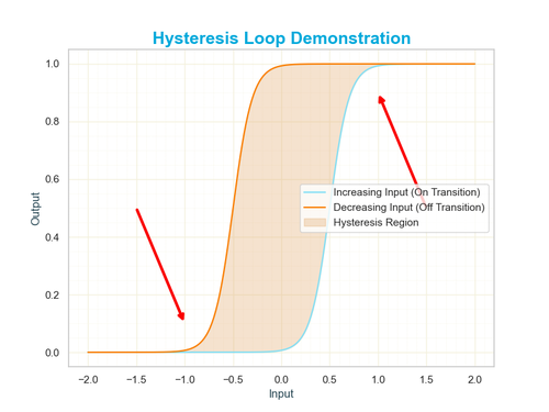
While the sigmoid function is known for its smooth, continuous transitions between two states, some systems require a more complex response. In certain cases, the output doesn’t just depend on the current input—it also depends on the system’s history. This phenomenon, known as hysteresis, introduces a form of memory into the system, creating a lag between changes in input and output. At first, hysteresis might seem unrelated to the predictable behavior of a sigmoid curve. However, the connection becomes clearer when considering how both functions model state transitions. A standard sigmoid responds immediately and symmetrically to changes in input, making it ideal for tasks like binary classification. In contrast, hysteresis reflects situations where the threshold for switching from one state to another depends on the input’s past behavior—such as a system that requires a higher input to switch "on" than to switch "off."

This memory effect is essential in real-world systems where stability and noise reduction are critical. For example, while a sigmoid function might represent the gradual likelihood of a decision being made, a hysteresis loop models systems that resist frequent switching due to minor fluctuations. The result is a curve with two distinct thresholds: one for activating a state and another for deactivating it. Below is an illustration of a typical hysteresis curve, highlighting how it differs from the smoother, more immediate transitions of a sigmoid.

Beyond machine learning, the sigmoid function plays a pivotal role in biological and psychological models of decision-making and growth. In neuroscience, for instance, the activation of neurons follows a pattern remarkably similar to the sigmoid curve. A neuron doesn’t fire unless its input exceeds a certain threshold, but once that happens, its firing rate increases rapidly before plateauing. This behavior mirrors the S-shaped progression of the sigmoid function, where small inputs produce minimal responses, moderate inputs trigger rapid increases, and large inputs level off at a maximum output. This resemblance to natural processes makes the sigmoid function a powerful tool for simulating biological systems and understanding how gradual shifts lead to significant outcomes.

Perhaps the most compelling reason for the sigmoid function’s importance is its role as a foundational concept in deep learning. While modern neural networks often use alternative activation functions, the sigmoid was one of the first to enable the training of multi-layered networks through techniques like backpropagation. Its smooth derivatives made it possible for algorithms to adjust their internal parameters efficiently, learning from data and improving over time. Although newer functions like ReLU have since taken precedence due to performance advantages, the sigmoid remains a critical concept for understanding the evolution of artificial intelligence. Its ability to translate complex, high-dimensional input data into manageable outputs continues to influence how modern systems are designed and optimized.

Understanding the sigmoid function

To truly understand the sigmoid function it helps to visualize how it behaves across different input values. The function itself is defined by a simple equation:

$$\sigma(x) = \frac{1}{1 + e^{-x}}$$

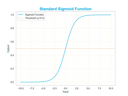
This formula might look intimidating at first, but its behavior is remarkably intuitive. The input \( x \) can be any real number—positive, negative, or zero. The exponential term \( e^{-x} \) ensures that for very large positive values of \( x \), the denominator becomes close to 1, making the output of the function approach 1. Conversely, for very large negative values of \( x \), the denominator grows exponentially, and the output approaches 0. The form of the function can be seen in the image shown on the right, below.

The most interesting behavior happens near \( x = 0 \). When \( x = 0 \), the equation simplifies to:

$$\sigma(0) = \frac{1}{1 + e^{0}} = \frac{1}{2}$$

This midpoint is critical because it represents the threshold of the sigmoid’s transition—where the output shifts from being closer to 0 to being closer to 1. Visually, this creates the S-shaped curve (also known as a logistic curve) that starts flat near 0, rapidly climbs around 0.5, and then flattens again near 1.

Imagine plotting the input values of \( x \) on a horizontal axis, with the output \( \sigma(x) \) on the vertical axis. As \( x \) moves from negative to positive, the curve rises smoothly from 0 to 1. This gradual transition reflects the function’s role in scenarios where outputs need to reflect probabilities or soft classifications rather than hard yes/no decisions. Small changes in \( x \) around the midpoint lead to significant shifts in the output, while larger values yield diminishing changes, effectively saturating the curve.

The steepness of the sigmoid curve can also be adjusted using a scaling parameter, often represented as \( k \) in a modified version of the equation:

$$\sigma(x) = \frac{1}{1 + e^{-kx}}$$

Here, \( k \) controls how quickly the transition from 0 to 1 occurs. A larger \( k \) value results in a steeper curve, causing outputs to shift rapidly with small changes in input—useful for situations where a sharp decision boundary is needed. Conversely, a smaller \( k \) value softens the curve, making transitions more gradual and allowing for greater uncertainty in decision-making.

Ultimately, visualizing the sigmoid function reveals its true strength: it’s not just about mapping numbers between 0 and 1, but doing so in a way that reflects how many real-world systems handle gradual changes. Whether it’s a neuron activating, a probability adjusting, or a system making a soft classification, the sigmoid function captures the essence of smooth transitions in complex systems.

Breaking Down the Maths (Gently)

At its heart, the sigmoid function is built on the foundations of exponential growth and decay, concepts that appear frequently in nature and mathematics. The key component of the function’s formula is the exponential term \( e^{-x} \), where \( e \) is Euler’s number (approximately 2.71828). This term is responsible for the smooth transition of the output, compressing extreme values of \( x \) into a manageable range between 0 and 1.

The full equation of the sigmoid function looks like this:

$$\sigma(x) = \frac{1}{1 + e^{-x}}$$

Let’s break it down step by step: - The input \( x \) can be any real number. - The negative sign in the exponent flips the input, making large negative values yield large positive exponents. - The exponential function \( e^{-x} \) ensures that large negative inputs will result in very large denominators, pushing the output closer to 0. - Adding 1 ensures that the denominator never reaches zero, keeping the output bounded between 0 and 1.

If we were to implement the sigmoid function in Python, it would look like this:

import math

def sigmoid(x):
    return 1 / (1 + math.exp(-x))

# Example usage
inputs = [-2, 0, 2]
outputs = [sigmoid(x) for x in inputs]
print(outputs)  # Output: [0.1192, 0.5, 0.8808]

This simple function takes an input \( x \), applies the exponential transformation, and outputs the corresponding sigmoid value. As you can see from the example, an input of 0 yields 0.5, confirming the sigmoid’s central threshold. Negative inputs approach 0, while positive inputs approach 1, but never quite reach either boundary, a concept known as asymptotic behaviour.

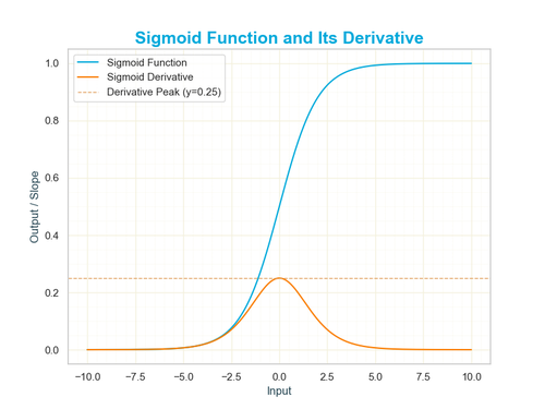
Another important feature of the sigmoid function is its derivative, which plays a crucial role in training machine learning models through backpropagation. The derivative is defined as:

$$\sigma'(x) = \sigma(x) \cdot (1 - \sigma(x))$$

This elegant result simplifies the maths for optimization algorithms. It tells us that the rate of change is greatest at \( x = 0 \), where the function is steepest, and diminishes as \( x \) moves toward extreme values, where the curve flattens. This behavior allows neural networks to make fine adjustments near decision boundaries while stabilizing outputs for more certain predictions.

Understanding both the function and its derivative helps explain why the sigmoid was historically favoured in early neural networks. While it’s been largely replaced by more efficient activation functions in modern deep learning, its mathematical clarity and intuitive behavior remain fundamental for grasping the foundations of machine learning.

Code Example - Implementing the Sigmoid Function

Now that we’ve explored the theory behind the sigmoid function, it’s time to implement it in code. Writing the function from scratch not only helps solidify your understanding of the math but also reveals how efficiently it can be used in practical applications like machine learning models. In this section, we’ll build a simple Python implementation and visualize how the function transforms input values.

Here’s a straightforward way to define the sigmoid function using Python’s built-in math library:

import math

def sigmoid(x):
    """Compute the sigmoid of x."""
    return 1 / (1 + math.exp(-x))

This function follows the mathematical definition of \( \sigma(x) = \frac{1}{1 + e^{-x}} \). The `math.exp(-x)` calculates the exponential term, while the division compresses the output to a value between 0 and 1. To verify that it works, we can pass a list of numbers through it and observe the output:

# Testing the sigmoid function
inputs = [-10, -2, 0, 2, 10]
outputs = [sigmoid(i) for i in inputs]

for i, o in zip(inputs, outputs):
    print(f"sigmoid({i}) = {o:.4f}")

You should expect the following output:

sigmoid(-10) = 0.0000
sigmoid(-2)  = 0.1192
sigmoid(0)   = 0.5000
sigmoid(2)   = 0.8808
sigmoid(10)  = 1.0000

As the results show, very negative values approach 0, very large positive values approach 1, and the midpoint \( x = 0 \) yields 0.5. This behaviour matches the theoretical properties we discussed earlier. Now, let’s take it one step further by visualizing the curve using the popular `matplotlib` library:

import matplotlib.pyplot as plt
import numpy as np

# Generate values from -10 to 10
x = np.linspace(-10, 10, 100)
y = [sigmoid(i) for i in x]

# Plotting the sigmoid curve
plt.plot(x, y)
plt.title("Sigmoid Function Curve")
plt.xlabel("Input Value (x)")
plt.ylabel("Sigmoid Output")
plt.grid(True)
plt.show()

This graph (which is shown earlier in the post) provides a clear visual of the sigmoid’s famous S-shaped curve. As expected, the output values approach 0 for large negative inputs and 1 for large positive inputs, with the steepest change occurring around \( x = 0 \). This sharp transition near the centre makes the sigmoid particularly useful in binary classification tasks, where models need to decide between two outcomes based on probability scores.

With this foundation in place, you now have both an intuitive understanding of the sigmoid function and a practical code implementation. This groundwork is essential for diving into more advanced applications, particularly in machine learning models where the sigmoid continues to play a foundational role.

Common Applications of the Sigmoid Function

The sigmoid function’s simplicity and smooth, predictable behaviour make it a versatile tool across various domains. Its ability to map any real-valued input into a constrained range between 0 and 1 is particularly valuable for scenarios where binary decisions or probability-based outputs are needed. From machine learning models to biological systems, the sigmoid function serves as a foundational element in both theoretical research and real-world applications.

One of the most common uses of the sigmoid function is in binary classification problems. In machine learning algorithms like logistic regression, the sigmoid function is used to convert a model’s output into a probability score. For instance, when determining whether an email is spam or not, the model produces a real-valued result, which the sigmoid function then transforms into a probability between 0 and 1. If the output is greater than a predefined threshold (often 0.5), the email is classified as spam; otherwise, it is not. This soft, probability-based output allows models to handle uncertainty more effectively than hard binary classifications.

The sigmoid function also plays a crucial role as an activation function in neural networks. Activation functions determine whether a particular neuron should “fire” based on its input. Early neural network architectures frequently used the sigmoid function because of its smooth gradient, which enabled efficient learning through backpropagation. This process adjusts the weights of connections between neurons based on how much error the output generates, with the sigmoid’s derivative helping guide these updates. Although other activation functions like ReLU have become more popular in modern deep learning due to performance benefits, the sigmoid remains essential for understanding the evolution of neural network design.

Beyond artificial intelligence, the sigmoid function appears in various biological models. In neuroscience, it’s often used to represent the firing rate of neurons. A neuron’s likelihood of firing increases with input but eventually plateaus, mirroring the sigmoid’s S-shaped curve. Similarly, in population biology, the sigmoid function models how populations grow in an environment with limited resources. Initially, growth is slow, accelerates rapidly as resources are plentiful, and then slows again as resources become scarce—a behaviour captured by the curve’s gradual rise and eventual saturation.

In economics and social sciences, the sigmoid function is used to model adoption rates of new technologies or behaviors. When a new technology is introduced, early adoption is typically slow. As awareness spreads and more people begin using the technology, adoption accelerates until it reaches a saturation point where nearly everyone who will adopt it has done so. This S-shaped growth pattern is a hallmark of innovation diffusion models and reflects the underlying dynamics of how trends spread through populations.

Even in fields like control systems and robotics, the sigmoid function is used for tasks that require smooth, non-linear scaling of input values. For example, it can help robots make gradual adjustments in movement or speed, avoiding sudden jerks that could destabilize the system. Its smooth output range makes it ideal for handling transitions where abrupt changes would be undesirable or dangerous.

Limitations of the Sigmoid Function

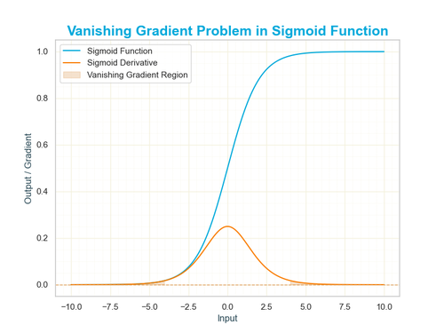
Despite its versatility the sigmoid function is not without its limitations, especially in the context of modern machine learning. One of the most significant issues is the vanishing gradient problem. When the input values become very large (positive or negative), the sigmoid function flattens out, and its derivative approaches zero. In deep neural networks, this can cause the gradients used for updating weights during training to become so small that the model stops learning altogether. As a result, networks that rely heavily on the sigmoid function can struggle with slow or incomplete convergence, particularly as more layers are added.

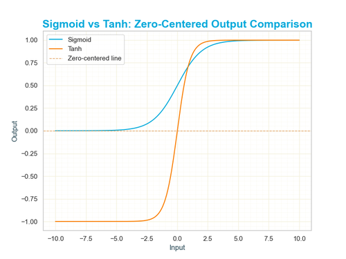
Another drawback lies in the function’s output range. Since the sigmoid outputs values strictly between 0 and 1, it is not zero-centred. This can lead to inefficient training in neural networks because the activations are always positive, which may result in undesirable patterns during optimization. Functions like the hyperbolic tangent (tanh), which outputs values between -1 and 1, help mitigate this issue by producing zero-centered outputs, leading to faster convergence and improved performance in many scenarios.

Lastly, the sigmoid function’s exponential calculation can be computationally expensive for large-scale machine learning models. While this isn’t typically an issue for small datasets or shallow networks, alternative activation functions like the Rectified Linear Unit (ReLU) have gained popularity due to their simplicity and computational efficiency. ReLU not only avoids the vanishing gradient problem for positive values but also requires fewer resources to compute, making it the preferred choice for deep learning applications. Despite these limitations, understanding the sigmoid function remains essential for grasping foundational concepts in machine learning and recognizing why newer alternatives were developed.

Why the Sigmoid Function Endures

While modern machine learning has largely moved toward newer activation functions like ReLU and its variants, the sigmoid function remains a cornerstone of the field. Its simplicity, mathematical elegance, and intuitive behavior make it an essential tool for understanding how more advanced models operate. Before diving into cutting-edge techniques, mastering the sigmoid function provides a strong foundation for grasping core concepts like probability mapping, non-linearity, and smooth decision boundaries.

Beyond machine learning, the sigmoid function continues to thrive in fields like biology, economics, and social sciences. Its ability to model gradual transitions and saturation effects makes it an invaluable tool for representing real-world systems, from population growth to technological adoption rates. These natural applications underscore the function’s versatility and highlight why it continues to be used in scientific research despite its computational limitations in deep learning.

Another reason for the sigmoid function’s enduring relevance is its interpretability. Unlike more complex models or functions, the sigmoid provides outputs that are easy to understand and interpret, particularly in probabilistic terms. This clarity makes it an excellent choice for applications where explainability is crucial—such as healthcare, finance, or regulatory environments—where stakeholders need to trust and understand a model’s decisions.

In the end, the sigmoid function’s legacy is not just about its role in early neural networks or its mathematical beauty. It represents a foundational concept that bridges simple intuition and complex systems, offering a gateway to deeper understanding in both artificial intelligence and natural phenomena. Whether you’re building a machine learning model, analyzing biological data, or exploring growth patterns, the sigmoid function remains a timeless tool for transforming complexity into clarity.

---